AFM Working Principle
The AFM principle is based on the cantilever/tip assembly that interacts with the sample; this assembly is also commonly referred to as the probe. The AFM probe interacts with the substrate through a raster scanning motion. The up/down and side to side motion of the AFM tip as it scans along the surface is monitored through a laser beam reflected off the cantilever. This reflected laser beam is tracked by a position-sensitive photo-detector (PSPD) that picks up the vertical and lateral motion of the probe. The deflection sensitivity of these detectors must be calibrated in terms of how many nanometers of motion correspond to a unit of voltage measured on the detector.
In order to achieve the AFM modes known as tapping modes, the probe is oscillated intermittently, bringing it in contact with the sample. There are two ways to oscillate the cantilever: 1) through a shaker piezo 2) through photothermal actuation (CleanDrive). The shaker piezo provides the ability to oscillate the probe at a range of frequencies (typically 100 Hz to 2 MHz). Photothermal excitation provides a cleaner and more stable actuation at an even wider range of frequencies (100 Hz to 8 MHz).
Tapping modes of operation can be categorized into resonant modes, where operation is at or near the resonance frequency of the cantilever, and off-resonance modes, where operation is at a frequency usually far below the cantilever’s resonance frequency.
The principle of how AFM works is depicted in the following schematic:

Photothermal actuation of AFM cantilevers - CleanDrive
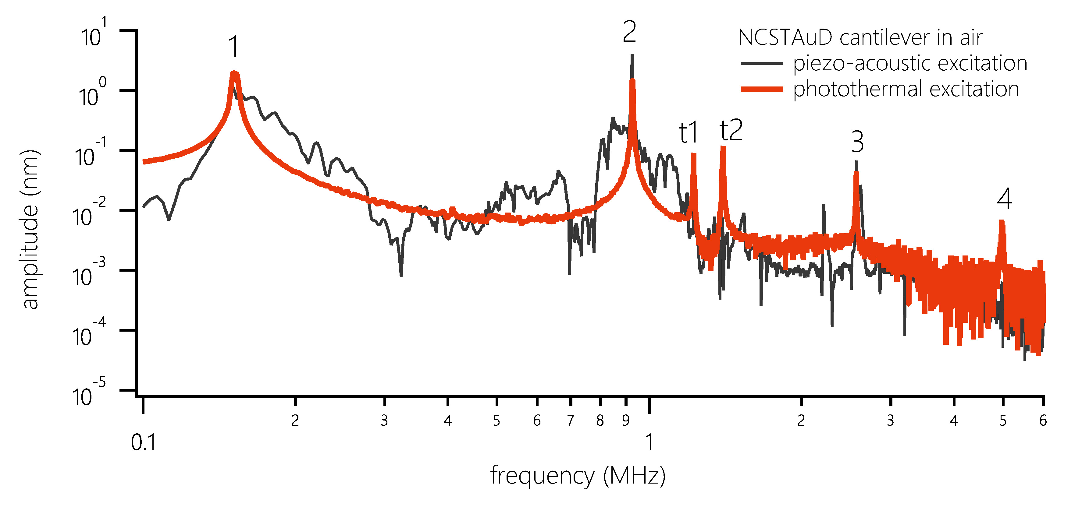
A direct way to actuate AFM cantilevers was introduced in 1991 [http://dx.doi.org/10.1116/1.585187], using photothermal excitation. It was included on the DriveAFM in 2020 as CleanDrive. Photothermal excitation offers significant improvement over conventional excitation of the AFM cantilevers by a “shaker piezo.” A shaker piezo vibrates not only the cantilever, but also the whole cantilever chip and cantilever holder assembly. This untargeted excitation beyond the cantilever can be a messy way to actuate the cantilever, particularly if the cantilever is immersed in an incompressible liquid with significant viscosity, like water. In water, piezo excitation results in a forest of peaks, in which the real cantilever resonance is hard to recognize. The height and frequency of those spurious peaks highly depend on the exact environment and are subject to change during operation. This results in reduced performance for many of the dynamic AFM modes.
Photothermal excitation provides very clean and focused actuation of just the cantilever by inducing a bimorph bending effect by local heating of the cantilever. Bimorph bending occurs due to different coefficients of thermal expansions for heterogeneous materials of the AFM cantilever - the silicon underside and the metal coating (typically Au or Al) on the top side, whose purpose is to enhance the reflectivity of the cantilever. Although photothermal excitation works with all commercial cantilevers in both air and fluid, coated cantilevers are preferred as they respond more strongly; gold-coated cantilevers are strongly recommended for fluid environments because of the limited stability of Al coatings in buffer solutions. An example of a frequency sweep of a cantilever in air is shown below using piezo actuation (black curve) and the photothermal actuation (red curve).
Cantilever/AFM tip assembly
This assembly consists of a very sharp tip (typical radius of curvature at the end for commercial tips is 5-10 nm) that hangs off the bottom of a long and narrow cantilever. As mentioned previously, the cantilever/tip assembly is also referred to as the AFM probe. The length/height of the AFM cantilever tip varies depending on the type of cantilever.
The two most common geometries for AFM cantilevers are rectangular ("diving-board") and triangular. An example of the diving board configuration of the levers is shown in the SEM image below; note the tip hanging off the end.

AFM cantilever material typically consists of either silicon or silicon nitride, where silicon nitride is reserved for softer cantilevers with lower spring constants. The dimensions of the cantilever are very important as they dictate its spring constant or stiffness. This stiffness is fundamental to governing the interaction between the AFM cantilever tip and the sample surface and can result in poor image quality if not chosen carefully. The relationship between the cantilever’s dimensions and spring constant, k, is defined by the equation:
k = Ewt 3 / 4L3,
where w = cantilever width; t = cantilever thickness; L = cantilever length and E = Young’s modulus of the cantilever material. Nominal spring constant values are typically provided by the vendor when buying the probes, but there can be significant variation in the actual values.
Nanosurf provides a straightforward manner of calibrating the spring constants of probes, which is described in the section below.
Deflection sensitivity calibration
The detector's sensitivity is calibrated to convert volts measured on the photodetector to nanometers of motion. The calibration is performed by measuring a force curve on an "infinitely stiff" surface such as sapphire. The "infinitely stiff" surface is chosen relative to the cantilever such that the cantilever does not indent the sample during the force curve measurement. Once the force curve of photodetector signal vs. piezo movement is collected, the slope of the repulsive portion of the wall is then calculated. This is the deflection sensitivity.

Note that on the Nanosurf Flex-ANA instrument and cantilever calibration options of other product lines this detector sensitivity calibration is automated, where multiple curves are collected and the average detector sensitivity value is calculated.
Spring constant calibration
Calibration of the spring constant of rectangular cantilevers is done via the Sader method on Nanosurf AFMs and implemented for all current product lines. This method relies on inputting the length and width of the cantilever (provided by the vendor and read from a cantilever list in the software). Generally, a thermal noise spectrum of the cantilever is recorded where the room temperature thermal motion is used to drive the cantilever. A sample thermal tuning spectrum is shown below. A single harmonic oscillator model is used to fit the peak in the thermal spectrum in order to extract the resonance frequency and quality factor. All these parameters are then input into the Sader model for hydrodynamic damping of the cantilever in a given environment, which then calculates the spring constant.
Alternatively, a frequency sweep can be used to calibrate the spring constant. Here the shaker piezo is used to drive the cantilever.
For spring constant calibration it is important that the cantilever is retracted from the surface when these frequency sweeps (either by thermal method or piezo) occur. A lift of at least 100 µm off the surface is recommended.

Feedback
The final principle that is important to understanding AFM operation is that of feedback. Feedback and feedback parameters are ubiquitous in our life. For example, temperature is the feedback parameter in a thermostat. A thermostat is set to the desired temperature (setpoint). As the temperature in the environment changes, it is compared with the temperature setpoint so that the heater (or air conditioner) knows when to turn on and off in order to keep the temperature at the desired value.
Similarly in atomic force microscopes, depending on the different modes, there is a parameter that serves as the setpoint. For example, in static mode (contact mode) the feedback parameter is cantilever deflection, while in the most common form of tapping mode, the cantilever oscillation amplitude is the feedback parameter. The instrument is trying to keep this feedback parameter constant at its setpoint value by adjusting the z-piezo to move the cantilever probe up and down. The resulting z-piezo movements provide the height information to create the surface topography.
Control of the feedback loop is done through the proportion-integral-derivative control, often referred to as the PID gains. These different gains refer to differences in how the feedback loop adjusts to deviations from the setpoint value, the error signal. For AFM operation, the integral gain is most important and can have a most dramatic effect on the image quality. The proportional gain might provide slight improvement after optimization of the integral gain. The derivative gain is mainly for samples with tall edges. If gains are set too low, the PID loop will not be able to keep the setpoint accurately. If the gains are chosen too high the result will be electrical noise in the image from interference from the feedback. The compensation for a deviation from the setpoint is larger than the error itself or noise gets amplified too strongly.
The other parameters that are important in feedback are the scan rate and the setpoint. If the scan rate is too fast, the PID loop will not have sufficient time to adjust the feedback parameter to its setpoint value and the height calculated from the z piezo movement will deviate from the true topography at slopes and near edges. Very slow scan rates are typically not an issue for the PID loop, but result in long acquisition times that can pose their own challenges such as thermal drift. Optimization of the PID gains and the scan rate are necessary in order to optimize feedback loops. The setpoint affects the interaction force or impuls between probe and sample. A setpoint close to the parameter value out of contact feedback is most gentle for the sample, but tends to slow down the feedback.
See below for an image that was collected with various PID gain settings at the same scan rate. In the red area the image is all electrical noise, because the gains are set too high. The area framed in orange also has some streaks of electrical noise illustrating the same problem. On the bottom, in the blue section, there is poor tracking due to gains being too low. A selected too high scan rate would have a similar appearance. The optimal image and parameter settings are in the green area.

Scanning
Electromagnetic scanners provide highly accurate and precise nanoscale motion in X, Y, and Z at low operation voltage in Nanosurf AFMs. These kinds of scanners provide significant advantages of highly linear motion and the absence of creep over other kinds of scanners such as piezoelectric scanners. The Nanosurf FlexAFM-based systems combine a piezoelectric scanner for Z motion with a flexure-based electromagnetic scanner in X and Y; this configuration provides fast motion in Z with maximum flatness in X and Y, which is optimal for the advanced capabilities offered by these systems.
Atomic force microscopes can be configured either to scan the tip over the sample (in which case the sample is stationary) or scan the sample under the tip (in which case the probe is stationary). All Nanosurf microscopes employ the tip scanning configuration. This configuration provides a significant advantage in terms of flexibility and size of the sample. Tip scanning instruments can accommodate large and unorthodox sample sizes; the only limitation on the sample is that it needs to fit into the instrument! Because the tip is moved and the sample remains stationary, the sample can be almost any size or weight and can still be scanned by the AFM. An example of sample flexibility is shown below with the NaniteAFM system and a custom-built translation/rotation stage to perform roughness measurements on large concave and convex samples.
